Artificial Intelligence and Machine Learning (AI/ML) have become a part of everything we do in our daily work. From personalised recommendations to automated decision-making, these technologies are everywhere. As AI/ML systems become more advanced, it’s crucial to ensure they are reliable and accurate. In this blog, we’ll explore simple and effective testing strategies to help improve these products, making them more trustworthy and high-quality.
Why this post?
Testing AI/ML projects can be challenging because models often seem like black boxes that produce outputs in ways that aren’t immediately clear. As a tester, how do you make sense of these models? Techniques like feature importance, Partial Dependence Plots, SHAP, and LIME can help. These techniques offer insights into how models make decisions, allowing us to better understand them. By gaining a clearer understanding of the models, we can design more effective tests and improve the quality of the systems we are working with.
Metamorphic testing
As testers, we typically expect a correct output based on the input of a test case. However, in the case of AI or ML systems, it’s not always possible to predict a specific output. For example, there is no guarantee that a specific product recommendation will appear based solely on a user’s search or purchase history. This uncertainty makes it difficult to define a ‘correct’ output, which is part of the test oracle problem. Metamorphic testing helps address this challenge by using properties of the system’s intended functionality. These properties, called metamorphic relations, must hold true across multiple executions of the software, even if the exact outputs are unknown. This concept will be illustrated with a practical example later in this post.
SHAP
SHapley Additive exPlanations (SHAP) shows how much each feature contributes to the final result. The SHAP value for each feature indicates how much that feature influences the prediction compared to a baseline. You can use SHAP for both global interpretation (overall model behaviour) and local interpretation (individual predictions) of the model. To understand about SHAP in detailed you can follow this link which has a Introduction page with examples.
Use Case
Now that we have some understanding of SHAP and Metamorphic tests, let’s use them to help test a model. We’ll create a sample model and use SHAP to identify the key features that influence its predictions. Assuming these key features are correct (a decision typically made by business experts and data analysts), we’ll design some Metamorphic tests. These tests can then be run each time the model is updated, ensuring that the relationships we expect to hold true still do. Here’s the plan:
– Build a sample model for illustration
– Use SHAP to analyze the model globally
– Design Metamorphic tests based on the analysis
– Run these tests on specific data to validate the model
Sample Model for Illustration
The sample model we developed predicts housing prices for a specific region in India. The dataset is from Kaggle and you can download it using the link here.
""" Script to train a machine learning model to predict the house price. """ import pandas as pd import numpy as np import optuna from sklearn.model_selection import train_test_split from sklearn.metrics import mean_squared_error from xgboost import XGBRegressor df = pd.read_csv('House_Price_India.csv') # Drop the 'id' and 'date' columns df = df.drop(columns=['id', 'Date']) def remove_outliers(data, column_name): ''' Function to detect outliers using IQR (Interquartile range) and remove them ''' first_quartile = df[column].quantile(0.25) third_quartile = df[column].quantile(0.75) interquartile_range = third_quartile - first_quartile lower_bound = first_quartile - 1.5 * interquartile_range upper_bound = third_quartile + 1.5 * interquartile_range data = data[(data[column_name] >= lower_bound) & (data[column_name] <= upper_bound)] return data #Remove outliers from specific columns columns_with_outliers = ['No of bedrooms', 'No of bathrooms', 'living area', 'lot area', 'No of views', 'house condition', 'house grade', 'house area(excluding basement)', 'Area of the basement', 'Price' ] for column in columns_with_outliers: df = remove_outliers(df, column) # Define features and target X = df.drop(columns=['Price']) y = df['Price'] # Split data X_train, X_test, y_train, y_test = train_test_split(X, y, test_size=0.2, random_state=42) def optimize_hyperparameters(trial): ''' Function to optimize hyperparameters''' param = { 'n_estimators': trial.suggest_int('n_estimators', 100, 1000), 'learning_rate': trial.suggest_float('learning_rate', 0.01, 0.3), 'max_depth': trial.suggest_int('max_depth', 3, 10), 'subsample': trial.suggest_float('subsample', 0.5, 1.0), 'colsample_bytree': trial.suggest_float('colsample_bytree', 0.5, 1.0), 'reg_alpha': trial.suggest_float('reg_alpha', 0, 1), 'reg_lambda': trial.suggest_float('reg_lambda', 0, 1) } model = XGBRegressor(objective='reg:squarederror', random_state=42, **param) model.fit(X_train, y_train) prediction = model.predict(X_test) optimized_rmse = np.sqrt(mean_squared_error(y_test, prediction)) return optimized_rmse study = optuna.create_study(direction='minimize') study.optimize(optimize_hyperparameters, n_trials=50) best_params = study.best_params print(f'Best hyperparameters: {best_params}') # Train the best model best_model = XGBRegressor(objective='reg:squarederror', random_state=42, **best_params) best_model.fit(X_train, y_train) # Evaluate the model y_pred = best_model.predict(X_test) rmse = np.sqrt(mean_squared_error(y_test, y_pred)) relative_rmse = (rmse / y_test.mean()) * 100 print(f'Bayesian Optimized XGBoost RMSE: {rmse}') print(f'Relative RMSE: {relative_rmse}%') mean_price = y_test.mean() median_price = y_test.median() print(f"Mean Price: {mean_price}, Median Price: {median_price}") |
Disclaimer: The code in this blog post is intended for demonstration purposes only. We recommend following better coding standards for real-world applications.
The steps include loading the dataset, preprocessing by removing outliers and splitting the data into training and testing sets. The model used is an XGBoost Regressor, and we perform some hyper parameter optimisation using Optuna to minimise the root mean squared error (RMSE). Finally, the best model is trained and evaluated, with performance metrics such as RMSE and relative RMSE reported.
The model achieved a Relative RMSE score of approximately 13% and an RMSE of around 56,300.
Bayesian Optimized XGBoost RMSE: 56318.88416126387 Relative RMSE: 13.072376951110584% |
Applying SHAP
In this section, we will see how we can apply SHAP to our model and gather some metamorphic test scenarios. We will first use SHAP for global interpretation and then for local interpretation.
Global Interpretation
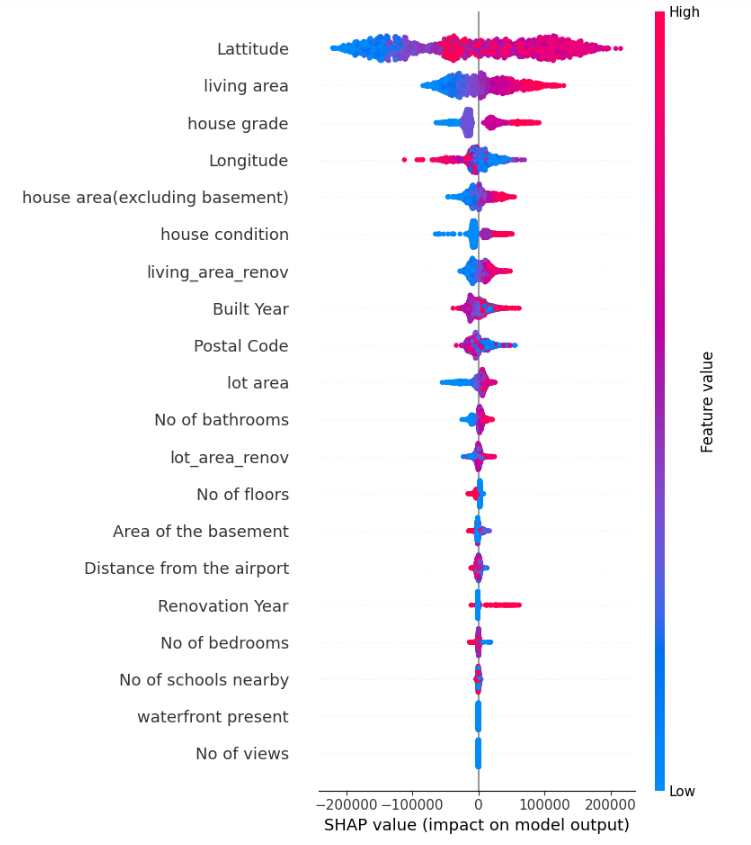
As discussed earlier, we can use SHAP for global interpretation. In this section, we analyse the model’s behaviour on a global scale. We begin by creating a SHAP explainer object using the trained model and then calculate SHAP values for the test data. These values provide insights into how each feature influences the model’s predictions. We will generate two types of summary plots:
– Summary Plot: Shows the impact of each feature on the model’s predictions, displaying the distribution of SHAP values across all samples.
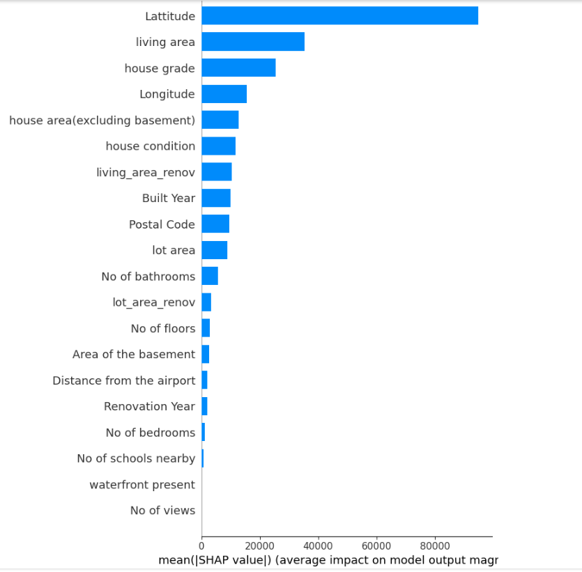
– Bar Plot: Ranks features by their overall importance, based on the average absolute SHAP values, helping us identify the most influential features in the model.
This global interpretation offers a comprehensive overview of the model’s decision-making process and highlights key features that significantly affect the predictions.
import shap import matplotlib.pyplot as plt import seaborn as sns # Create a SHAP explainer object explainer = shap.Explainer(best_model, X_train) # Calculate SHAP values shap_values = explainer(X_test) # Summary plot of SHAP values with feature names shap.summary_plot(shap_values, X_test, feature_names=X.columns) # Bar plot of SHAP feature importances with feature names shap.summary_plot(shap_values, X_test, plot_type="bar", feature_names=X.columns) |
 |
 |
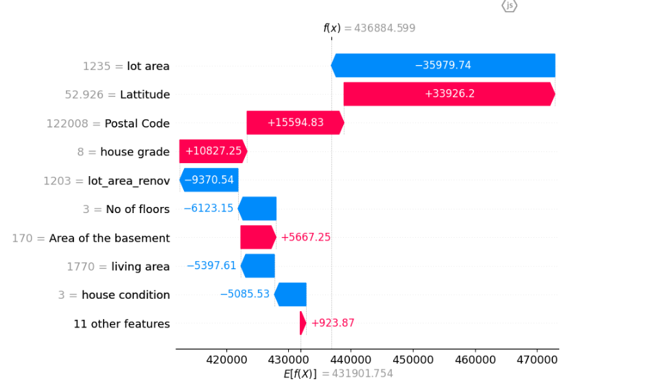
Local Interpretation
For local interpretation, SHAP helps us understand a model’s prediction for a specific instance by breaking down the contribution of each feature. In this example, we use a specific dataset from our data to illustrate local interpretation. We calculate SHAP values for the data point and visualise them using a force plot and a waterfall plot. These plots show how each feature influenced the prediction, either pushing it higher or lower relative to the model’s baseline.
instance_data = { 'No of bedrooms': 3, 'No of bathrooms': 2.5, 'living area': 1770, 'lot area': 1235, 'No of floors': 3, 'waterfront present': 0, 'No of views': 0, 'house condition': 3, 'house grade': 8, 'house area(excluding basement)': 1600, 'Area of the basement': 170, 'Built Year': 2007, 'Renovation Year': 0, 'Postal Code': 122008, 'Lattitude': 52.9265, 'Longitude': -114.532, 'living_area_renov': 1680, 'lot_area_renov': 1203, 'No of schools nearby': 3, 'Distance from the airport': 52 } instance_df = pd.DataFrame([instance_data]) # Create a SHAP explainer object explainer = shap.Explainer(best_model, X_train) # Calculate SHAP values shap_values = explainer(instance_df) shap.initjs() # Local interpretation for the specific instance shap.force_plot(explainer.expected_value, shap_values.values[0], instance_df.iloc[0], feature_names=X.columns) # Waterfall plot for better visualization of contributions shap.waterfall_plot(shap_values[0]) # Actual price actual_price = 436110 # Predict Price for the instance data predicted_log_price = best_model.predict(instance_df) print(f"Predicted Log Price: {predicted_log_price}") # Print the original actual price for comparison print(f"Original Actual Price: {actual_price}") |
Disclaimer: In this example, all data is declared directly in the code to make the example easy to understand. Ideally, we would read this data from a file and use it for analysis.
Building Metamorphic test Scenarios
Now that we understand the important features and how to use local interpretation, we can design some metamorphic tests. The global analysis highlighted latitude, house grade, and living area as key features. We’ll create tests to verify the following:
– Latitude and Living Area: Adjusting these values upwards or downwards should result in an increase or decrease in the predicted price.
– Waterfront Present and Number of Views: SHAP analysis indicates that these features have no impact on the model’s predictions, which is unexpected as they should typically affect house prices. We will add tests to confirm this finding
These metamorphic tests are crucial as they act as reliable checks. For instance, increasing or decreasing important features should positively or negatively affect the predicted price. They provide a dependable way to ensure the model’s accuracy and should be included in your regression tests to confirm that the model works correctly after any updates.
Results
Lets examine the results
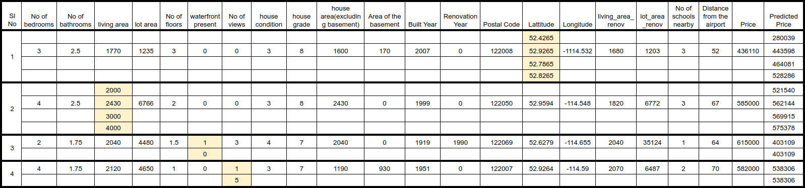
- By plotting Latitude against price, we can identify which Latitude values are associated with higher or lower prices. I selected one row from the dataset and adjusted its Latitude value to observe changes in the predicted price, keeping all other features constant. As shown in the image above, the results revealed that less desirable Latitude values resulted in lower predicted prices, while better Latitude values led to higher predicted prices. This test scenario effectively illustrates the impact of Latitude on the model’s predictions.
- In the second scenario, I adjusted the Living Area to observe its effect on the predicted price. The results demonstrate that changes in Living Area do influence the predictions, with increasing the area leading to a higher predicted price and decreasing it resulting in a lower predicted price. However, the change in predicted price isn’t very substantial; for instance, doubling the Living Area from 2,000 to 4,000 resulted in an increase in the predicted price from 521,540 to 575,378. This relatively modest change suggests that while Living Area does affect predictions, its impact appears limited. This could indicate a potential issue with the model, and further analysis may be needed to understand and address this.
- In the third and fourth scenarios, I adjusted the Waterfront present and No of Views features. As previously shown by the SHAP analysis, these features had no noticeable impact on the predicted price. This suggests there may be a problem with the model, possibly due to limited data for these features.
Conclusion
Even though machine learning models can seem like black boxes, it’s important for testers to find ways to gain insights into their inner workings. Using tools like SHAP and methods like metamorphic testing, we can better understand and validate the model’s behaviour. This makes sure the model performs well in real life and gives us a clearer picture of why it behaves the way it does. The more we understand and share about the model, the more confidence stakeholders will have in its results.
References:
1. Opening the Black Box of Machine Learning Models: SHAP vs LIME for Model Explanation
Hire QA from Qxf2 Services
At Qxf2, we have skilled technical testers who are well versed in both traditional and modern testing methods. We specialise in testing microservices, data pipelines, and AI/ML applications. Our engineers are great at working independently and in small teams. Contact us here for more information.

I am a dedicated quality assurance professional with a true passion for ensuring product quality and driving efficient testing processes. Throughout my career, I have gained extensive expertise in various testing domains, showcasing my versatility in testing diverse applications such as CRM, Web, Mobile, Database, and Machine Learning-based applications. What sets me apart is my ability to develop robust test scripts, ensure comprehensive test coverage, and efficiently report defects. With experience in managing teams and leading testing-related activities, I foster collaboration and drive efficiency within projects. Proficient in tools like Selenium, Appium, Mechanize, Requests, Postman, Runscope, Gatling, Locust, Jenkins, CircleCI, Docker, and Grafana, I stay up-to-date with the latest advancements in the field to deliver exceptional software products. Outside of work, I find joy and inspiration in sports, maintaining a balanced lifestyle.